CoCAS is a standalone Chromatin immunoprecipitation
microarray (ChIP-on-chip) analysis application. It has been designed to be
used primarily on Agilent microarrays scanned with an Agilent scanner.
CoCAS is free software and builds upon
existing packages in Java and R programming languages, notably BioConductor.
CoCAS uses Java for user graphical interface, and
R for the bulk of the calculations.
CoCAS can be readily started by double
clicking on the CoCAS_2.4.jar icon. Alternatively, CoCAS may be run from the
command line with specific parameters, for example, in order to assign more
memory to CoCAS, one would type java -Xmx2048m -jar [path to
CoCAS]/CoCAS_2.4.jar . A welcome screen will prompt you to use the
express wizard, which is an easy step by step guide.

Upon first use, you should click "No" so
that you can check that you have all the required libraries. You can
do this by clicking on the "Libraries" menu item from the "Update" menu.
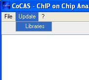
CoCAS will then check and download libraries
where appropriate. This process can be quite lengthy.
1. Guided Wizard
CoCAS features a simple wizard that can help
you design your analysis. There are eight steps which provide detailed help.
The first step is to define an analysis name. Then comes file loading which
is explained in the next section.
2. Loading
Files
Files can be loaded three ways in CoCAS. One
way is to use the step-by-step guided wizard, or from the main window,
either by right clicking on the File Panel, or by using the File Menu. In
the classic mode, once you have loaded files, the main panel, which was
greyed out, becomes accessible. CoCAS allows you to enter all replicas of a
same experiment under one slide. For example, if you have two
replicas of one experiment, 252040810001 and 252040810002, you will enter
them under slide 1 for example
3. Dye Swap
Dye-swap
normally sets Cy3 to the IP channel and Cy5 to the Input
channel.
4. Intra-array normalization
parameters
You can here choose from four normalization methods :
Median normalization
assumes that the red and green intensities are related by a constant factor,
i.e. R = kG, and the center of the distribution of log ratios is shifted to
zero
log2R/G -> log2R/G � c = log2R/(kG)
where
c = log2k is the median.
See Zien A, Aigner T, Zimmer
R, Lengauer T. Centralization: a new method for the normalization of gene
expression data. Bioinformatics. 2001;17 Suppl 1:S323-31. for details
Lowess (Locally weighted
scatter plot smoothing) intensity-dependent normalization performs a fit of
the data by subtracting a linear regression curve.
log2R/G ->
log2R/G � c(A) = log2R/[k(A)G]
where c(A) is the lowess fit to the
MA-plot.
See Yang YH, Dudoit S, Luu P,
Lin DM, Peng V, Ngai J, Speed TP. Normalization for cDNA microarray data: a
robust composite method addressing single and multiple slide systematic
variation. Nucleic Acids Res. 2002 Feb 15;30(4):e15. for details
The Variance Stabilisation
Normalisation (V.S.N.) method builds upon the fact that the
variance of microarray data depends on the signal intensity and that a
transformation can be found after which the variance is
approximately constant. See Huber W, von Heydebreck
A, S�ltmann H, Poustka A, Vingron M. Variance stabilization applied to
microarray data calibration and to the quantification of differential
expression. Bioinformatics. 2002;18 Suppl 1:S96-104. for details
Peng et al.
normalization uses signal enrichment rotation against
intensity according to an angle estimated by PCA, then applies a weighted
loess normalization. See Peng S, Alekseyenko AA,
Larschan E, Kuroda MI, Park PJ. Normalization and experimental design for
ChIP-chip data. BMC Bioinformatics. 2007 Jun 25;8:219. for details
5. Multiple Slide
Designs
High density microarray designs can
sometimes be spread over more than one slide, i.e. in the case of whole
genome experiments.
This option causes all slides entered as one
experiment to be treated as replicates of part of a multi-slide
design.
Example:
251471611301 : chr1-10 Replicate 1 as slide
1
251471611302 : chr1-10 Replicate 2 as slide 1
251471711301 : chr11-Y
Replicate 1 as slide 2
251471711302 : chr10-Y Replicate 2 as slide 2
Multiple
slide designs are handled as separate experiments until inter array
normalization, after which they are merged as whole experiment.
6. Inter-array normalization
parameters
You can here choose from three normalization methods :
-
None
-
Median
-
Quantile
-
Peng et al.
Quantile normalization is based upon the concept of a quantile-quantile plot extended to n dimensions. No special allowances are made for outliers. See Bolstad, B. M., R. A. Irizarry, M. Astrand, and T. P. Speed. 2003. A comparison of normalization methods for high density oligonucleotide array data based on variance and bias. Bioinformatics. 19(2):185-193. for more details
Global median normalization achieves the same median signal intensities for each array. See Bolstad, B. M., R. A. Irizarry, M. Astrand, and T. P. Speed. 2003. A comparison of normalization methods for high density oligonucleotide array data based on variance and bias. Bioinformatics. 19(2):185-193. for more details
7. Replicate Merging Method
You can here choose two methods :
Mean merging method simply calculates the mean of intensities for each probe on all arrays
Roberts et al. uses the Rosetta error model Weng, L., H. Dai, Y. Zhan, Y. He, S. B. Stepaniants, and D. E. Bassett. 2006. Rosetta error model for gene expression analysis. Bioinformatics. 22(9):1111-1121. for more details
Back to Home